A billing forecast curve allows you to divide anticipated revenue over a series of sequences of time in a larger time period (such as a quarter). You can define billing forecast curves on the following:
- The billing forecast setup
- A project
- An opportunity
The billing forecast curve is made up of a number of billing forecast curve details, or points on the curve, each covering a certain number of days (Period) and indicating the percentage of the total forecast amount to apply during that period (Percent Burndown).
A billing forecast curve is basically a delivery schedule you can build, based on how your business typically performs.
For information on creating billing forecast curves, see Managing Curves for Billing Forecasts.
Billing forecast curve data is stored in the Billing Forecast Curve and Billing Forecast Curve Detail objects. For more information, see:
Examples
Applying a Billing Forecast Curve to a Project
A billing forecast curve is set on a project that spans Quarter 2 (Q2). The billing forecast curve is configured as follows:
- Lag = 10 days (applies from the run date of the billing forecast calculation and delays the start of burndown)
- Curve Detail 1 = Sequence: 1; Period: 20 days; Percent Burndown: 20%
- Curve Detail 2 = Sequence: 2; Period: 30 days; Percent Burndown: 80%
The length of the curve is the sum of the Lag and the Periods set on the curve details = 60 days.
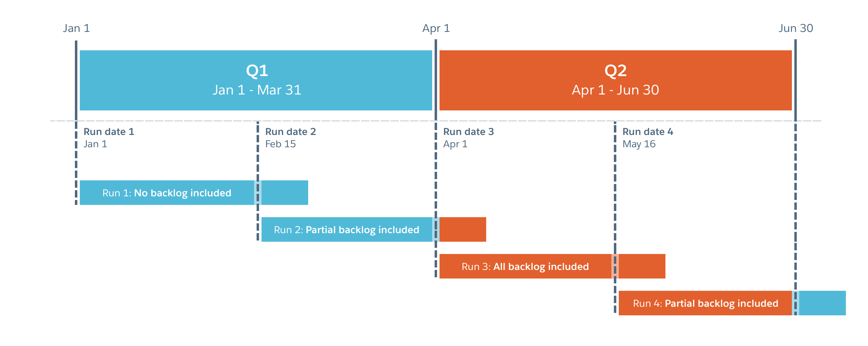
The Q2 billing forecast calculation is run four times: on January 1, February 15, April 1, and May 16.
Run 1: January 1
January 1 + 60 days = March 1
Unscheduled backlog forecast = 0%
As January 1 does not fall within the Q2 time period, no unscheduled backlog is included in the billing forecast calculation.
Run 2: February 15
Feb 15 + 60 days = April 16
Unscheduled backlog forecast = 42.67%
As 16 days of the curve fall within the Q2 time period, only part of the unscheduled backlog is included in the billing forecast calculation.
Run 3: April 1
April 1 + 60 days = May 30
Unscheduled backlog forecast = 100%
As both the forecast run date and the curve end date fall within the Q2 time period, all of the unscheduled backlog is included in the billing forecast calculation.
Run 4: May 16
May 16 + 60 days = July 15
Unscheduled backlog forecast = 40%
As 45 days of the curve fall within the Q2 time period, only part of the unscheduled backlog is included in the billing forecast calculation.
The following diagram shows what is included in each run:
Applying a Billing Forecast Curve to an Opportunity
We take the weighted opportunity value and then project the delivery based on a curve that you apply to one of the following:
- The total opportunity amount
- The products that you would use on the opportunity
Weighted value of opportunity: value in Amount field multiplied by Probability % = $10,000
Projected close date = January 1.
The business typically delivers a project over the following duration:
- Month 1 after opportunity close date = 0% delivered
- Month 2 = 10% delivered
- Month 3 = 30% delivered
- Month 4 = 30% delivered
- Month 5 = 20% delivered
- Month 6 = 10% delivered
The billing forecast curve reflects this delivery pattern:
- January = $0
- February = $1,000
- March = $3,000
- April = $3,000
- May = $2,000
- June = $1,000
 SECTIONS